The common practice of estimating the probability of entire risk scenarios as a whole is prone to gross error, particularly when arbitrarily numbered incremental category scales are employed (see Take the red pill). So in a previous posting (Some realities of risk) I introduced the concept of the risk factor tree as an alternative tool for improving the reliability of scenario risk assessment. I‘ll now go one step further and show how to actually calculate the probability of a scenario from its factor tree.
Defining probability
We first need a reliable definition of probability, and there’s none better than that of Abraham de Moivre. A French mathematician who settled in England in the late 1680s, de Moivre had the rare gift of being able to express mathematical ideas in plain language, and he wrote in English rather than the Latin preferred by his contemporaries.
I quote the first two sentences from the 1756 edition of de Moivre’s very readable book The Doctrine of Chances:[1]
‘The Probability of an Event is greater or less, according to the number of Chances by which, it may happen, compared with the whole number of Chances by which it may either happen or fail.
Wherefore, if we constitute a Fraction whereof the Numerator be the number of Chances whereby an Event may happen, and the Denominator the number of all the Chances whereby it may either happen or fail, that Fraction will be a proper designation of the Probability.’ Clearly, the number times an event happens can never be greater than the number of opportunities for it to happen – de Moivre’s ‘all the Chances whereby it may either happen or fail’. Consequently the value of probability can never exceed one. It also follows logically that if the probability of something happening is x, the probability of it not happening is 1–x. For example, if a brilliant golfer were to score a hole in one on average every 50 drives, the probability of her doing so would be 1/50 or 0.02 (two per cent) and the probability of her missing would be 49/50 or 0.98 (98 per cent). So goodbye scale of one to five, hello scale of zero to one. Combining probabilities But why does this matter? As the probability of an outcome depends on the probabilities of its (often multiple) causal factors, to calculate the probability of the outcome we must be able to combine the probabilities of those factors. Provided we represent probability on the range of zero to one it’s surprisingly simple, but if we use arbitrary numbers such as one to five the math fails, yielding apparent results that are nevertheless nonsense. Once we accept this, there are two basic principles. First, a causal factor has two alternatives - it can either happen or not. So for a set of some number (let’s say n) of factors, there are two to the power of n possible logical ways for them to combine (each either occurring or not occurring).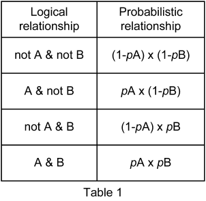 Column one of table 1 shows these logical combinations for the simplest case of just two factors (represented by A and B), but the same principle can be extended to any number of factors by working out the full set of all their possible combinations. You might note a similarity of the logical combinations in column one to binary number representation, and you’d be right.
Column two shows the equivalent probabilities, where pA and pB represent the probabilities of A and B respectively. We owe the relationships between the logical combinations and the probabilities to George Boole’s brilliant if turgid 1853 book An investigation of the laws of thought, on which are founded the mathematical theories of logic and probabilities.[2]
The second principle is that there are two fundamental ways that factors can combine to result in an outcome. If several factors must all occur together for an outcome to result, the relationship is logical AND (also represented by the symbol ‘&’). However if several factors may occur in any combination to result in the outcome but any one of them alone is sufficient, the relationship is logical OR.
Courtesy of Boole, if any number of factors are in an AND relationship, we simply multiply their probabilities to obtain their aggregate probability.
However for the OR relationship, aggregate probability is calculated differently. Row one of Table 1 represents the condition where neither factor occurs so the outcome doesn’t happen, but to obtain the overall probability of the outcome occurring we must combine the probabilities of the three alternative combinations of factors that can cause it to happen (rows two, three and four of table 1). Another of Boole’s rules is that provided multiple events in an OR relationship are strict alternatives – a logical Exclusive OR relation – their probabilities should be added together to obtain their aggregate probability. As all the rows of table 1 are indeed mutually exclusive, we could calculate the probabilities of the three combinations that result in the outcome (A & not B, not A & B, A & B) and add them together. However for each additional factor the number of combinations doubles (binary numbers again), so the calculation can get cumbersome.
When we eventually come to combine likelihoods with consequences to derive risk we’ll need to consider all the alternative combinations of factors separately, but as at the moment we’re only interested in the overall probability of our scenario happening there’s a simpler way. Remembering that the probability of something not happening is just one minus the probability of it happening, the probability that any of the three alternative ways our two OR-related factors can cause the scenario is just one (certainty it will occur) minus the probability than neither factor occurs (not A & not B – the first row of table 1).
Column one of table 1 shows these logical combinations for the simplest case of just two factors (represented by A and B), but the same principle can be extended to any number of factors by working out the full set of all their possible combinations. You might note a similarity of the logical combinations in column one to binary number representation, and you’d be right.
Column two shows the equivalent probabilities, where pA and pB represent the probabilities of A and B respectively. We owe the relationships between the logical combinations and the probabilities to George Boole’s brilliant if turgid 1853 book An investigation of the laws of thought, on which are founded the mathematical theories of logic and probabilities.[2]
The second principle is that there are two fundamental ways that factors can combine to result in an outcome. If several factors must all occur together for an outcome to result, the relationship is logical AND (also represented by the symbol ‘&’). However if several factors may occur in any combination to result in the outcome but any one of them alone is sufficient, the relationship is logical OR.
Courtesy of Boole, if any number of factors are in an AND relationship, we simply multiply their probabilities to obtain their aggregate probability.
However for the OR relationship, aggregate probability is calculated differently. Row one of Table 1 represents the condition where neither factor occurs so the outcome doesn’t happen, but to obtain the overall probability of the outcome occurring we must combine the probabilities of the three alternative combinations of factors that can cause it to happen (rows two, three and four of table 1). Another of Boole’s rules is that provided multiple events in an OR relationship are strict alternatives – a logical Exclusive OR relation – their probabilities should be added together to obtain their aggregate probability. As all the rows of table 1 are indeed mutually exclusive, we could calculate the probabilities of the three combinations that result in the outcome (A & not B, not A & B, A & B) and add them together. However for each additional factor the number of combinations doubles (binary numbers again), so the calculation can get cumbersome.
When we eventually come to combine likelihoods with consequences to derive risk we’ll need to consider all the alternative combinations of factors separately, but as at the moment we’re only interested in the overall probability of our scenario happening there’s a simpler way. Remembering that the probability of something not happening is just one minus the probability of it happening, the probability that any of the three alternative ways our two OR-related factors can cause the scenario is just one (certainty it will occur) minus the probability than neither factor occurs (not A & not B – the first row of table 1).
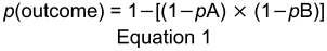 Equation 1 represents this simple formula, which delivers a single result expressing the probability of an outcome resulting from any combination of two causal factors in an OR relationship. It can be extended to accommodate any number of OR-related factors simply by multiplying in a (1–p) term derived from the probability of each additional factor.
Calculating scenario probability
These two calculations can be applied to any tree of causal factors leading to a single scenario. But how in practice? The answer is - incrementally.
We built a factor tree (Some realities of risk) iteratively from a scenario through successive tiers of causal factors until we reached a leaf factor on every branch - a factor either for which causal factors could not be identified or over the causes of which no control could be exercised, but, in either case, for which some estimate of probability could be made. Examples might include third party service failures, lightning strikes, the likelihood that an email is SPAM or the relative prevalence of a specific cyber attack vector.
Equation 1 represents this simple formula, which delivers a single result expressing the probability of an outcome resulting from any combination of two causal factors in an OR relationship. It can be extended to accommodate any number of OR-related factors simply by multiplying in a (1–p) term derived from the probability of each additional factor.
Calculating scenario probability
These two calculations can be applied to any tree of causal factors leading to a single scenario. But how in practice? The answer is - incrementally.
We built a factor tree (Some realities of risk) iteratively from a scenario through successive tiers of causal factors until we reached a leaf factor on every branch - a factor either for which causal factors could not be identified or over the causes of which no control could be exercised, but, in either case, for which some estimate of probability could be made. Examples might include third party service failures, lightning strikes, the likelihood that an email is SPAM or the relative prevalence of a specific cyber attack vector.
 Having built the (upside down) tree from its root (the scenario) to its leaves, we reverse the direction to calculate the scenario probability, starting from the leaf factors and working iteratively towards the scenario at the root.
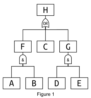
In figure 1, A and B (in an AND relation) are leaf factors causing F, and D and E (in an AND relation) are leaf factors causing G. The root scenario H is then caused by any combination of F (the outcome of A and B) or G (the outcome of D and E) or leaf factor C.
First, we assign probability values for the leaf factors of the tree, based on available evidence. From those, we’ll use the simple math we‘ve discussed to calculate successive probability values towards the root depending on the logical relationships between the factors. Thus we calculate pF from assigned values for pA and pB, and pG from assigned values for pD and pE. Then we calculate pH (the scenario probability) from the assigned value for pC and the previously calculated values for pF and pG.
Plugging in some numbers
To keep the arithmetic simple for this demonstration, we’ll assign the notional values pA = 0.1, pB = 0.2, pC = 0.3, pD = 0.4 and pE = 0.5, although the real world probabilities of individual factors are typically a lot lower. For example, the probability of a ‘once a year’ event occurring on any given day is 1/365 or about 0.0027.
Step one is to multiply the probabilities of the AND-related factor pairs (A & B, D & E).
Having built the (upside down) tree from its root (the scenario) to its leaves, we reverse the direction to calculate the scenario probability, starting from the leaf factors and working iteratively towards the scenario at the root.
In figure 1, A and B (in an AND relation) are leaf factors causing F, and D and E (in an AND relation) are leaf factors causing G. The root scenario H is then caused by any combination of F (the outcome of A and B) or G (the outcome of D and E) or leaf factor C.
First, we assign probability values for the leaf factors of the tree, based on available evidence. From those, we’ll use the simple math we‘ve discussed to calculate successive probability values towards the root depending on the logical relationships between the factors. Thus we calculate pF from assigned values for pA and pB, and pG from assigned values for pD and pE. Then we calculate pH (the scenario probability) from the assigned value for pC and the previously calculated values for pF and pG.
Plugging in some numbers
To keep the arithmetic simple for this demonstration, we’ll assign the notional values pA = 0.1, pB = 0.2, pC = 0.3, pD = 0.4 and pE = 0.5, although the real world probabilities of individual factors are typically a lot lower. For example, the probability of a ‘once a year’ event occurring on any given day is 1/365 or about 0.0027.
Step one is to multiply the probabilities of the AND-related factor pairs (A & B, D & E).
Director, BiR
10/09/2022
Wherefore, if we constitute a Fraction whereof the Numerator be the number of Chances whereby an Event may happen, and the Denominator the number of all the Chances whereby it may either happen or fail, that Fraction will be a proper designation of the Probability.’ Clearly, the number times an event happens can never be greater than the number of opportunities for it to happen – de Moivre’s ‘all the Chances whereby it may either happen or fail’. Consequently the value of probability can never exceed one. It also follows logically that if the probability of something happening is x, the probability of it not happening is 1–x. For example, if a brilliant golfer were to score a hole in one on average every 50 drives, the probability of her doing so would be 1/50 or 0.02 (two per cent) and the probability of her missing would be 49/50 or 0.98 (98 per cent). So goodbye scale of one to five, hello scale of zero to one. Combining probabilities But why does this matter? As the probability of an outcome depends on the probabilities of its (often multiple) causal factors, to calculate the probability of the outcome we must be able to combine the probabilities of those factors. Provided we represent probability on the range of zero to one it’s surprisingly simple, but if we use arbitrary numbers such as one to five the math fails, yielding apparent results that are nevertheless nonsense. Once we accept this, there are two basic principles. First, a causal factor has two alternatives - it can either happen or not. So for a set of some number (let’s say n) of factors, there are two to the power of n possible logical ways for them to combine (each either occurring or not occurring).
Column one of table 1 shows these logical combinations for the simplest case of just two factors (represented by A and B), but the same principle can be extended to any number of factors by working out the full set of all their possible combinations. You might note a similarity of the logical combinations in column one to binary number representation, and you’d be right.
Column two shows the equivalent probabilities, where pA and pB represent the probabilities of A and B respectively. We owe the relationships between the logical combinations and the probabilities to George Boole’s brilliant if turgid 1853 book An investigation of the laws of thought, on which are founded the mathematical theories of logic and probabilities.[2]
The second principle is that there are two fundamental ways that factors can combine to result in an outcome. If several factors must all occur together for an outcome to result, the relationship is logical AND (also represented by the symbol ‘&’). However if several factors may occur in any combination to result in the outcome but any one of them alone is sufficient, the relationship is logical OR.
Courtesy of Boole, if any number of factors are in an AND relationship, we simply multiply their probabilities to obtain their aggregate probability.
However for the OR relationship, aggregate probability is calculated differently. Row one of Table 1 represents the condition where neither factor occurs so the outcome doesn’t happen, but to obtain the overall probability of the outcome occurring we must combine the probabilities of the three alternative combinations of factors that can cause it to happen (rows two, three and four of table 1). Another of Boole’s rules is that provided multiple events in an OR relationship are strict alternatives – a logical Exclusive OR relation – their probabilities should be added together to obtain their aggregate probability. As all the rows of table 1 are indeed mutually exclusive, we could calculate the probabilities of the three combinations that result in the outcome (A & not B, not A & B, A & B) and add them together. However for each additional factor the number of combinations doubles (binary numbers again), so the calculation can get cumbersome.
When we eventually come to combine likelihoods with consequences to derive risk we’ll need to consider all the alternative combinations of factors separately, but as at the moment we’re only interested in the overall probability of our scenario happening there’s a simpler way. Remembering that the probability of something not happening is just one minus the probability of it happening, the probability that any of the three alternative ways our two OR-related factors can cause the scenario is just one (certainty it will occur) minus the probability than neither factor occurs (not A & not B – the first row of table 1).
Equation 1 represents this simple formula, which delivers a single result expressing the probability of an outcome resulting from any combination of two causal factors in an OR relationship. It can be extended to accommodate any number of OR-related factors simply by multiplying in a (1–p) term derived from the probability of each additional factor.
Calculating scenario probability
These two calculations can be applied to any tree of causal factors leading to a single scenario. But how in practice? The answer is - incrementally.
We built a factor tree (Some realities of risk) iteratively from a scenario through successive tiers of causal factors until we reached a leaf factor on every branch - a factor either for which causal factors could not be identified or over the causes of which no control could be exercised, but, in either case, for which some estimate of probability could be made. Examples might include third party service failures, lightning strikes, the likelihood that an email is SPAM or the relative prevalence of a specific cyber attack vector.
Having built the (upside down) tree from its root (the scenario) to its leaves, we reverse the direction to calculate the scenario probability, starting from the leaf factors and working iteratively towards the scenario at the root.
In figure 1, A and B (in an AND relation) are leaf factors causing F, and D and E (in an AND relation) are leaf factors causing G. The root scenario H is then caused by any combination of F (the outcome of A and B) or G (the outcome of D and E) or leaf factor C.
First, we assign probability values for the leaf factors of the tree, based on available evidence. From those, we’ll use the simple math we‘ve discussed to calculate successive probability values towards the root depending on the logical relationships between the factors. Thus we calculate pF from assigned values for pA and pB, and pG from assigned values for pD and pE. Then we calculate pH (the scenario probability) from the assigned value for pC and the previously calculated values for pF and pG.
Plugging in some numbers
To keep the arithmetic simple for this demonstration, we’ll assign the notional values pA = 0.1, pB = 0.2, pC = 0.3, pD = 0.4 and pE = 0.5, although the real world probabilities of individual factors are typically a lot lower. For example, the probability of a ‘once a year’ event occurring on any given day is 1/365 or about 0.0027.
Step one is to multiply the probabilities of the AND-related factor pairs (A & B, D & E).
As pA = 0.1 and pB = 0.2, pF = 0.02
As pD = 0.4 and pE = 0.5, pG = 0.2
As pC = 0.3, 1–pC = 0.7
As pF = 0.02, 1–pF = 0.98
As pG = 0.2, 1–pG = 0.8
REFERENCES
[1] Reproductions of the 1756 third edition of The Doctrine of Chances are available free from several online sources
[2] Reproductions of Boole's An investigation of the laws of thought are available free from several online sources
Mike Barwise
[1] Reproductions of the 1756 third edition of The Doctrine of Chances are available free from several online sources
[2] Reproductions of Boole's An investigation of the laws of thought are available free from several online sources
Director, BiR
10/09/2022
A version of this article appeared in CIISec Pulse, May 2022